
Simulating Your First Operational Risk#
Real-world deployments expose AI models to environmental and sensor-level degradations that rarely appear in training data. Validating robustness to these conditions is a core part of Artificial Intelligence Test & Evaluation (AI T&E).
In this guide, you’ll use NRTK’s
JitterPerturber
to apply a physics-based jitter perturbation that simulates high-frequency
vibration — the kind of sensor blur caused by wind, vehicle movement, or
mechanical instability on mounted cameras. By the end, you’ll be able to:
Understand what an operational risk perturbation looks like in practice
See how a few lines of code can simulate a real-world degradation
Get a feel for NRTK’s perturbation workflow before exploring more perturbers
When to Use This#
You want to simulate platform vibration from wind, vehicle movement, or mechanical instability.
You need a physics-based perturbation that models realistic motion blur effects.
You’re doing early screening of robustness to vibration before running heavier T&E analysis (see the full T&E Simulation Guide → JitterPerturber T&E guide).
You want to test model performance at reduced effective resolution due to motion.
Example: Jitter Perturbation#
Important
JitterPerturber requires the pybsm extra. If you haven’t already, install it:
pip install nrtk[pybsm]
See Installation for alternatives.
The following example loads an image, applies a jitter perturbation, and saves the result:
from nrtk.impls.perturb_image.optical.otf import JitterPerturber
import numpy as np
from PIL import Image

# Load your image
image = np.array(Image.open("your_image.jpg"))

# Apply jitter perturbation
# img_gsd = ground sample distance (meters/pixel) for your sensor
perturber = JitterPerturber(s_x=8e-6, s_y=8e-6)
perturbed_image, _ = perturber(image=image, img_gsd=0.03)

# Save the result
Image.fromarray(perturbed_image).save("perturbed_output.jpg")
The s_x and s_y parameters control jitter amplitude — see
Key Parameters below for details and visual comparisons.
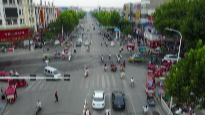
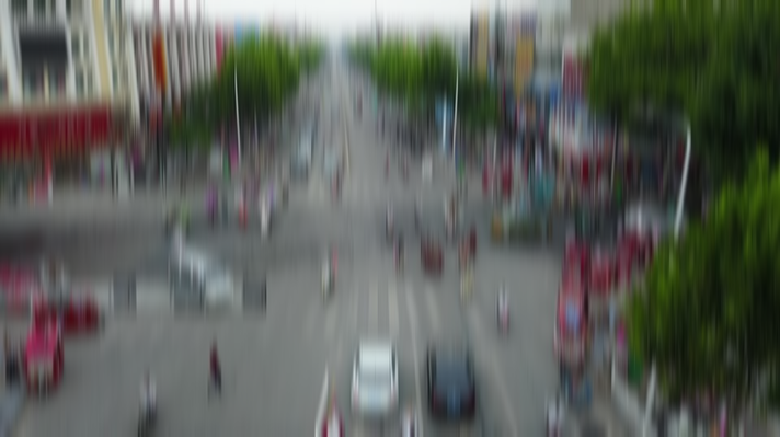
Here’s what the perturbation looks like in practice:
Baseline Image (No Jitter) |
Image with Simulated Sensor Jitter |
|---|---|

|
|
Notice how the jitter perturbation introduces motion blur that reduces edge sharpness and suppresses fine detail. In deployed systems, this kind of degradation can increase missed detections, reduce confidence scores, and lower mAP — precisely the kinds of robustness gaps T&E aims to surface before fielding. The severity of this degradation is controlled by the jitter amplitude parameters, explored below.
Key Parameters#
s_x,s_y— Root-mean-squared jitter amplitudes in x and y directions (radians). These represent the standard deviation of angular positional error due to platform vibration. Larger values produce a stronger Gaussian blur.Light (0, 3e-4)
Medium (0, 5e-4)
Heavy (0, 1e-3)

See also
For a deeper dive into optical perturber parameters and OTF modeling, see the Optical Perturbers notebook.
Other Operational Risks#
NRTK provides perturbers for a range of real-world degradations beyond vibration. Each module below includes a description, code example, parameter comparison, and links to further resources.
Simulates reduced visibility from fog, mist, or light snow.
Simulates blur and distortion from unstable air masses.
Simulates under- or overexposure from harsh lighting conditions.
Simulates optical defocus from autofocus failures or focus errors.
Simulates barrel or pincushion distortion from wide-angle lenses.
Simulates thermal noise, electronic noise, and resolution loss.
Simulates lens contamination from rain or water spray.
References#
API Reference:
JitterPerturberFull Explanation: High-Frequency Vibration Module — Physics background, OTF modeling details, and limitations
T&E Simulation Guide: JitterPerturber T&E guide — Detailed analysis, validation, datasets, and recommended parameter sweeps
End-to-End Tutorial: NRTK End-to-End Overview — Complete workflow covering perturbation, factories, and model evaluation
Concepts: Concepts of Robustness in Computer Vision — Conceptual guide to NRTK’s architecture and approach
Risk Matrix: Operational Risk Factors in Computer Vision — Map real-world operational risks to NRTK perturbations