
Applying an Operational Risk Perturbation#
In real-world deployments, cameras mounted on vehicles, drones, or handheld platforms experience vibration that blurs images and degrades model performance. Most vision models are trained on clean, stable imagery, leading to even mild jitter causing missed detections or poor accuracy.
In this guide, you’ll use NRTK’s JitterOTFPerturber to apply your first physics-based perturbation and see how sensor jitter affects an image. This is a good starting point if you want to:
Understand what an operational risk perturbation looks like in practice
See how a few lines of code can simulate a real-world degradation
Get a feel for NRTK’s perturbation workflow before exploring more perturbers
Example: Jitter Perturbation#
In this example, we’ll apply a jitter perturbation to an image. Afterwards, the NRTK tutorial provides a deeper look at perturbations and the other main components of NRTK.
Input Image#
Below is an example of an input image that will undergo a Jitter perturbation. This image represents the initial state before any transformation.
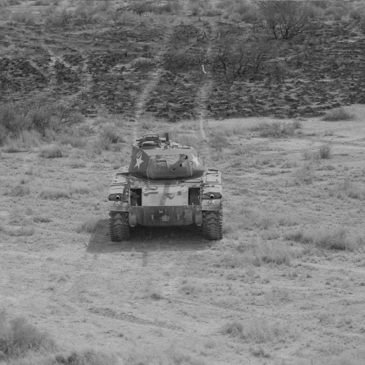
Figure 1: Input image.#
Code Sample#
Below is some example code that applies a Jitter OTF transformation:
from nrtk.impls.perturb_image.optical.otf import JitterPerturber
import numpy as np
from PIL import Image

INPUT_IMG_FILE = 'docs/images/input.jpg'
image = np.array(Image.open(INPUT_IMG_FILE))

otf = JitterPerturber(s_x=8e-6, s_y=8e-6)
out_image = otf(image=image)
This code uses default values and provides a sample input image. However, you can adjust the parameters and use your
own image to visualize the perturbation. The s_x and s_y parameters (the root-mean-squared jitter amplitudes in
radians, in the x and y directions) are the primary way to customize a jitter perturber. Larger jitter amplitudes
generate a larger Gaussian blur kernel. The
how-to guide on OTF perturbations will provide more detail on selecting
specific values for these parameters.
Resulting Image#
The output image below shows the effects of the Jitter perturbation on the original input. This result illustrates the Gaussian blur introduced due to simulated sensor jitter.

Figure 2: Output image.#
Next Steps#
Now that you’ve applied a single perturbation, the NRTK End-to-End Overview walks through a complete workflow—image perturbation, perturbation factories, and model evaluation.
For broader context or foundational theory, see:
High-Frequency Vibration Module — Full operational risk details, parameter sweeps, and visual comparison
Concepts of Robustness in Computer Vision — Conceptual guide to NRTK’s architecture and approach
Operational Risk Factors in Computer Vision — How NRTK’s perturbations map to real-world risk factors