NRTK Overview Tutorial

Introduction

NRTK consists of two main parts:

1. Image Perturbation

2. Perturbation Factories

If you’re unfamiliar with these components, see the NRTK Overview page for brief descriptions before continuing.

The following sections will guide you through setting up and using an example perturber. By the end of this tutorial, you’ll have a working example that you can expand for your own projects.

To run this notebook in Colab, use the link below:

Note for Colab users: After setting up the environment, you may need to “Restart Runtime” in order to resolve package version conflicts (see the README for more info).

Prerequisites

Before starting, ensure the following:

• NRTK is installed (see Installation).

• Software Requirements:

  • Supported Python versions:

  • pip (Python package manager) installed.

• Basic Skills: Familiarity with Python programming and using the terminal or command line.

The following sections will guide you through setting up and using an example perturber.

%pip install -qU pip
print("Installing nrtk...")
try:
    import pybsm  # noqa: F401 -- intentionally unused, just checking availability

    import nrtk  # noqa: F401 -- intentionally unused, just checking availability
except ImportError:
    %pip install -q "nrtk[pybsm]"
    pass  # jupytext converts %pip to a comment, so pass keeps the block valid
print("Done")

Note: you may need to restart the kernel to use updated packages.
Installing nrtk...
Done

Image Perturbation

The core of NRTK is based on image perturbation. NRTK offers a wide variety of ways to perturb images. Libraries such as scikit-image, Pillow, openCV, and pyBSM are used for various types of perturbation. The perturbation classes take an image and perform a transformation based on input parameters. The examples shown below focus on a pyBSM based perturber.

For this example, we are going to use the PybsmPerturber from pyBSM. This perturber is useful for creating new images based on existing parameters.

We’ve preselected parameter values for the sensor and scenario objects for this tutorial, but this pyBSM explanation covers image formation concepts that provide insight into how these parameters are selected.

import copy

import numpy as np
from pybsm.otf import dark_current_from_density

from nrtk.impls.perturb_image.optical import PybsmPerturber

opt_trans_wavelengths = np.array([0.58 - 0.08, 0.58 + 0.08]) * 1.0e-6
f = 4  # telescope focal length (m)
p = 0.008e-3  # detector pitch (m)
sensor_config = {
    # required
    "sensor_name": "L32511x",
    "D": 275e-3,  # Telescope diameter (m)
    "f": f,
    "p_x": p,
    "opt_trans_wavelengths": opt_trans_wavelengths,  # Optical system transmission, red  band first (m)
    # optional
    "optics_transmission": 0.5
    * np.ones(opt_trans_wavelengths.shape[0]),  # guess at the full system optical transmission (excluding obscuration)
    "eta": 0.4,  # guess
    "w_x": p,  # detector width is assumed to be equal to the pitch
    "w_y": p,  # detector width is assumed to be equal to the pitch
    "int_time": 30.0e-3,  # integration time (s) - this is a maximum, the actual integration time will be,
    # determined by the well fill percentage
    "dark_current": dark_current_from_density(
        jd=1e-5,
        w_x=p,
        w_y=p,
    ),  # dark current density of 1 nA/cm2 guess, guess mid range for a silicon camera
    "read_noise": 25.0,  # rms read noise (rms electrons)
    "max_n": 96000,  # maximum ADC level (electrons)
    "bit_depth": 11.9,  # bit depth
    "max_well_fill": 0.6,  # maximum allowable well fill (see the paper for the logic behind this)
    "s_x": 0.25 * p / f,  # jitter (radians) - The Olson paper says that its "good" so we'll guess 1/4 ifov rms
    "s_y": 0.25 * p / f,  # jitter (radians) - The Olson paper says that its "good" so we'll guess 1/4 ifov rms
    "qe_wavelengths": np.array([0.3, 0.4, 0.5, 0.6, 0.7, 0.8, 0.9, 1.0, 1.1]) * 1.0e-6,
    "qe": np.array([0.05, 0.6, 0.75, 0.85, 0.85, 0.75, 0.5, 0.2, 0]),
}

scenario_config = {
    "scenario_name": "niceday",
    "ihaze": 1,  # weather model
    "altitude": 9000.0,  # sensor altitude
    "ground_range": 0.0,  # range to target
    "aircraft_speed": 100.0,
}

sensor_and_scenario_config = sensor_config | scenario_config

updated_config = copy.deepcopy(sensor_and_scenario_config)
updated_config["ground_range"] = 10000

perturber = PybsmPerturber(**updated_config)

./.tox/papermill/lib/python3.10/site-packages/tqdm/auto.py:21: TqdmWarning: IProgress not found. Please update jupyter and ipywidgets. See https://ipywidgets.readthedocs.io/en/stable/user_install.html
  from .autonotebook import tqdm as notebook_tqdm

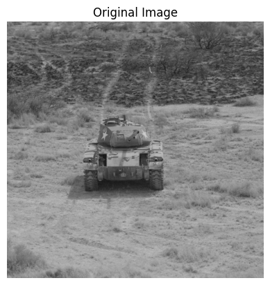
In the example above, we have created a pyBSM perturber where the output image will have a ground_range of 10000m instead of 0m. The image below is the original image we will use for future perturbations.

Note: ground_range refers to the projection of line of sight between the camera and target along on the ground (in meters).

import os
import urllib.request
import warnings

import cv2
import matplotlib.pyplot as plt

warnings.filterwarnings("ignore")

data_dir = "./data"
os.makedirs(data_dir, exist_ok=True)

url = "https://data.kitware.com/api/v1/item/6596fde89c30d6f4e17c9efc/download"

img_path = os.path.join(data_dir, "M-41 Walker Bulldog (USA) width 319cm height 272cm.tiff")
if not os.path.isfile(img_path):
    _ = urllib.request.urlretrieve(url, img_path)  # noqa: S310

img = cv2.imread(img_path)
if img is None:
    raise FileNotFoundError(f"Failed to load image: {img_path}")

fig, ax = plt.subplots()
ax.imshow(img)
ax.set_title("Original Image")
ax.set_axis_off()

The code block below shows the loading of the image above and the calling of the perturber. It is important to note that the Ground Sample Distance (or img_gsd) is another parameter the user will have to provide. The resulting image is displayed below the code block.

Note: GSD (Ground Sample Distance) is the distance between the centers of two adjacent pixels in an image, measured on the ground. A smaller GSD (more pixels per ground area) means a higher resolution image, capturing more detail. Conversely, a larger GSD (fewer pixels per ground area) means a lower resolution image, capturing less detail.

img_gsd = 3.19 / 165.0  # the width of the tank is 319 cm and it spans ~165 pixels in the image
perturbed_image, _ = perturber(image=img, img_gsd=img_gsd)

fig, ax = plt.subplots()
ax.imshow(perturbed_image)
ax.set_title("Perturbed Image")
ax.set_axis_off()

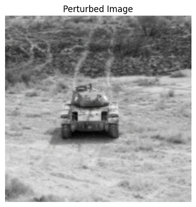
From the perturbed image above, we can observe a blurred output image. It is important to note that this is simulated by a sensor with a telescope focal length (f) of 4 metres, detector pitch (p) of 8 millimeters and telescope diameter (D) of 275 millimeters. In the given scenario, the sensor is at 9000 meters above ground level (altitude) mounted on an aircraft moving at 100 meters per second (aircraft_speed).

Any of the parameters in either sensor_config or scenario_config can be modified; however, the PybsmPerturber basic perturber can modify only a single parameter for each instance call. The next section will cover modifying multiple parameters and multiple values using perturber factories.

Perturbation Factories

Continuing on from the previous example, the snippet below shows the initialization of a PerturberMultivariateFactory. The theta_keys variable controls which parameter(s) we are modifying and thetas are the actual values of the parameter(s). In this example, we are modifying the focal length (f) with the values of 1, 2, and 3. The modified images are displayed below the code block.

from nrtk.impls.perturb_image_factory import PerturberMultivariateFactory

focal_length_pf = PerturberMultivariateFactory(
    perturber=PybsmPerturber,
    theta_keys=["f"],
    thetas=[[1, 2, 3]],
    perturber_kwargs=sensor_and_scenario_config,
)

_, ax = plt.subplots(1, 3, figsize=(10, 4))
for idx, perturber in enumerate(focal_length_pf):
    perturbed_img, _ = perturber(image=img, img_gsd=img_gsd)
    ax[idx].set_title(f"focal_length: {idx + 1}")
    ax[idx].imshow(perturbed_img)
    _ = ax[idx].axis("off")
plt.tight_layout()

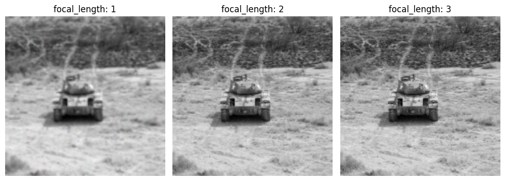
From the generated output images above, we can observe that as focal length increases from 1 to 3 meters, a sharper image of the tank is generated indicating that, comparatively, a focal length of 3 meters is preferable to get a sharper image of the tank.

Using the PerturberMultivariateFactory, it is possible to assign series of values to one or more parameters simultaneously. Each PerturberMultivariateFactory instance consists of a series of individual perturber instances based on the number of parameter-value combinations.

The code block below shows the focal length and ground range variables being modified. The resulting images are displayed below the code block.

import itertools

f_groung_range_pf = PerturberMultivariateFactory(
    perturber=PybsmPerturber,
    theta_keys=["f", "ground_range"],
    thetas=[[1, 2], [10000, 20000]],
    perturber_kwargs=sensor_and_scenario_config,
)
perturber_factory_config = f_groung_range_pf.get_config()
if "theta_keys" in perturber_factory_config:  # pyBSM doesn't follow interface rules
    perturb_factory_keys = perturber_factory_config["theta_keys"]
    thetas = f_groung_range_pf.thetas
else:
    perturb_factory_keys = [f_groung_range_pf.theta_key]
    thetas = [f_groung_range_pf.thetas]
perturber_combinations = [dict(zip(perturb_factory_keys, v, strict=False)) for v in itertools.product(*thetas)]

_, ax = plt.subplots(1, 4, figsize=(10, 4))
for idx, perturber in enumerate(f_groung_range_pf):
    perturbed_img, _ = perturber(image=img, img_gsd=img_gsd)
    ax[idx].set_title(
        f"focal_length: {perturber_combinations[idx]['f']}\n"
        f"ground_range: {perturber_combinations[idx]['ground_range']}",
    )
    ax[idx].imshow(perturbed_img)
    _ = ax[idx].axis("off")
plt.tight_layout()

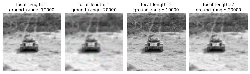
In the above images, it is important to note that the simulation does not follow a linear progression as seen in the prior example. When modifying multiple parameters simultaneously, we can observe drastic changes in the image texture (blurring and subsampling effects) as we sweep through to find the optimal combination for the f (focal_length) and ground_range parameters.

Model Evaluation

NRTK’s image perturbation tools are often used in conjuction with evaluation workflows such as Modular AI Trustworthy Engineering (MAITE), which support modular test configuration and scoring. If you’re working within a JATIC ecosystem or evaluating robustness as scale, tools like MAITE help integrate perturbations into end-to-end pipelines. See our Testing & Evaluation (T&E) Guides for tutorials on evaluating models against operational risks using NRTK and MAITE.

Next Steps

Now that you’ve completed this tutorial, you can:

• Explore Advanced Features: Try different perturbation methods.

• Use Larger Datasets: Test NRTK on real-world datasets.

See pages under the How-To Guides section for more details on applying various perturbations.

See pages under the Reference section for code documentation.

See the pyBSM documentation for explanatory information regarding the theory behind perturbations, jitter effects, and the significance of certain parameters.