
Concepts of Robustness in Computer Vision#
Computer vision models are highly sensitive to data distribution shifts, which can arise from either:
Synthetic image perturbations (e.g., artificially applied noise, blur, or transformations) [1].
Naturally occurring variations in real-world data, such as changes in lighting, sensor properties, or environmental conditions [2].
The Challenge of Robustness Testing#
The gold standard for evaluating AI model robustness is to test against diverse real-world datasets that fully cover the expected range of deployment conditions. However:
Collecting exhaustive test data is prohibitively expensive and, in some cases, impossible.
Many critical conditions (e.g. varying sensor properties) cannot be easily captured in real-world datasets.
Standard augmentation libraries fall short. Existing image augmentation libraries, such as imgaug and albumentations, provide useful transformations like rotation, scaling, and noise addition, but do not account for the physics-based, sensor-specific perturbations that are crucial for evaluating how AI models perform in real-world operational conditions.
How NRTK Helps#
The Natural Robustness Toolkit (NRTK) enables principled robustness testing by augmenting finite test datasets with realistic, physics-based perturbations.
- This allows AI practitioners to:
Simulate real-world variations that would occur due to different imaging conditions.
Evaluate AI model performance under conditions that are difficult to replicate with standard data collection.
Optimize sensor design for AI-based detection and classification tasks.
Figure 1 illustrates how NRTK integrates into a typical model evaluation workflow. It highlights where NRTK’s physics-based test data augmentation is positioned within the broader pipeline — between training and robustness assessment — providing a way to generate expanded datasets that reflect realistic imaging conditions. These expanded datasets enable more meaningful and interpretable robustness evaluation by simulating variations in sensor parameters and environmental conditions that are complex or expensive to capture in real-world data.
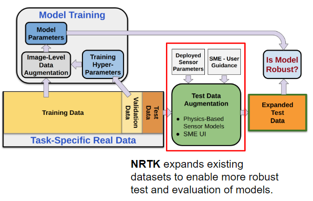
Figure 1: Extending Robustness Testing with NRTK.#
The following sections explain the types of sensor-specific perturbations that NRTK can simulate and how these are applied and evaluated within an AI pipeline.
Understanding Sensor-Specific Perturbations in AI Robustness#
NRTK specializes in sensor-specific perturbations, enabling more realistic robustness evaluation than standard augmentations. These perturbations model how changes in imaging sensor parameters affect AI models.
Key Sensor-Based Perturbations#
- NRTK can simulate variations in:
Focal length – Alters the effective field of view and spatial resolution.
Aperture size – Impacts depth of field and light collection.
Pixel pitch – Affects sensor resolution and noise characteristics.
Quantum efficiency – Determines how efficiently photons are converted to electrical signals.
Compression and noise effects – Models artifacts introduced by storage and transmission.
These perturbations are particularly useful in applications where AI performance depends on imaging conditions, such as satellite imagery, surveillance, and autonomous systems.
How NRTK Works: Image Perturbation#
Image Perturbations#
- NRTK applies controlled image perturbations to assess model robustness. These perturbations are implemented using:
Pre-sensor modeling – Adjusts scene parameters before the image is captured.
In-sensor effects – Simulates sensor distortions (e.g., noise, blur, quantization).
Post-sensor processing – Models compression artifacts and other downstream effects.
NRTK integrates with pyBSM, an open source library that rigorously models radiative transfer and imaging-sensor physics [3]. This allows for highly realistic perturbations tailored to specific sensor configurations. It also provides functionality through Strategy and Adapter patterns to allow for modular integration into systems and applications.
Model Evaluation#
After perturbing images, practitioners can gain insights into how robust AI models are to real-world sensor variations via model evaluation. NRTK is interoperable with MAITE (as well as the remainder of the JATIC tools!) and together these tools enable teams to develop more reliable vision based AI-systems by:
Testing model performance using perturbed datasets.
Comparing model outputs across different perturbation settings.
Supporting classification and detection tasks in a black-box manner.
Interpreting Robustness Results#
NRTK generates performance curves that show how model behavior changes with increasing perturbation strength. Understanding how to interpret these results is critical for making informed decisions about model robustness.
Understanding Perturbation Parameters#
Increasing parameter values (e.g., blur sigma, noise amplitude, ground range) represent progressively stronger degradations or more challenging imaging conditions.
Parameter ranges should reflect realistic operational bounds. For example, ground-range variations should correspond to actual deployment scenarios, not arbitrary numerical sweeps.
Linear vs. non-linear effects: Single-parameter sweeps often show monotonic performance changes, but multi-parameter sweeps can exhibit complex interactions where the effect is non-additive.
Effective limits: Some parameters reach saturation points where further increases produce negligible additional degradation (e.g., extreme blur, where the model has already lost any useful signal).
Reading Performance Curves#
Performance curves plot model metrics (accuracy, precision, recall, mAP) against perturbation strength:
Steep drops indicate sensitivity to that perturbation type - a potential operational vulnerability that warrants investigation or mitigation.
Gradual degradation suggests robustness; the model degrades predictably as imaging conditions worsen, which is often acceptable for operational use.
Performance cliffs (sudden drops at specific parameter values) are particularly concerning as they indicate narrow operating ranges in which small changes in conditions cause large performance impacts.
Plateau regions show where the model has reached its failure threshold; additional perturbation doesn’t further degrade performance because the model has already lost critical information.
Non-monotonic curves (performance improving then declining) may indicate overfitting to specific conditions or unexpected model behavior worth investigating.
Comparing Models#
When evaluating multiple models under identical perturbations, consider the following factors:
Consistent performance advantage: Performance across perturbation strengths indicates greater robustness, though this should be verified with operational data before making deployment decisions.
Crossover points: When one model outperforms another at different perturbation levels, this suggests different robustness profiles. Consider which conditions are most operationally relevant.
Perturbation-specific sensitivity: Models often show different vulnerabilities (e.g., robust to blur but sensitive to noise). Map these sensitivities to operational risk factors to prioritize concerns.
Divergence magnitude: Differences between models under perturbation reveal how much robustness varies; small differences may not be operationally significant even if statistically measurable.
Material vs. Nominal Changes#
Determining whether a performance change requires action depends on operational context:
Material change: Performance drop exceeds mission-critical thresholds (e.g., >5% accuracy loss, unacceptable missed detections). Requires mitigation strategies or operational constraints.
Nominal change: Performance remains within acceptable operational bounds. May warrant monitoring but doesn’t require immediate intervention.
Define thresholds before testing: What constitutes “material” depends on mission requirements, not NRTK. Establish acceptable performance ranges based on operational consequences before running experiments.
Task-specific interpretation: A 2% detection accuracy drop might be nominal for vehicle counting but material for threat identification. Consider the trade-offs between false positives and negatives for your specific application.
Statistical vs. practical significance: Statistically significant changes may not be operationally meaningful if they fall within acceptable performance bounds.
Integration with Operational Risk Assessment#
NRTK results inform but do not replace operational validation:
Link to risk factors: Connect observed sensitivities to operational conditions using the Operational Risk Factors in Computer Vision mapping. If a model is sensitive to jitter perturbations, consider vibration risks in your deployment environment.
Prioritize validation efforts: Use NRTK to identify which perturbation types cause material performance changes, then prioritize collecting real-world data for those specific conditions.
Communicate uncertainty: NRTK perturbations are approximations of real-world effects. Present results as “indicative of potential sensitivity” rather than “proof of operational failure.”
Iterative refinement: Use initial NRTK screening to guide data collection, then validate findings with operational data and refine your understanding of model robustness.
For additional context on when NRTK results should inform decisions versus when additional validation is needed, see validation_and_trust.
NRTK Algorithms#
The NRTK algorithms can be organized according to their respective tasks:
- Image perturbation:
- MAITE interoperability:
Interoperability
References#
Hendrycks, Dan, and Thomas Dietterich. “Benchmarking Neural Network Robustness to Common Corruptions and Perturbations.” International Conference on Learning Representations. 2018.
Recht, Benjamin, et al. “Do imagenet classifiers generalize to imagenet?.” International Conference on machine learning. PMLR, 2019.
LeMaster, Daniel A., and Michael T. Eismann. 2017. “pyBSM: A Python package for modeling imaging systems.” Proceedings of the SPIE 10204.