Demonstrating Rain/Water Droplet Perturbations

Introduction

This notebook is part of the NRTK demonstration suite, demonstrating how perturbations can be applied and their impact measured via MAITE evaluation workflows.

Layout

This notebook demonstrates how a particular condition (in this case, Rain or Water droplets), can affect an object detection model, and how that impact can be measured. The overall structure is:

• Evaluation Guidance: Computing Mean Average Precision (mAP):

  • An overview of the evaluation strategy.

• Setup:

  • Notebook initialization, loading the supporting python code. Depending on if this is the first time you’ve run this notebook, this may take some time.

  • Loading the source image, which will be used throughout the notebook.

• Image Perturbation Examples:

  • The NRTK perturbation is demonstrated on the source image.

• Baseline Detections:

  • The object detection model is loaded and run on the unperturbed image. These will serve as “ground truth” for comparisons against the perturbed images.

At this point, we have the fundamental elements of our evaluation: the model, our reference image, and a mechanism for creating the perturbed test images. Next we adapt these elements to be used with the MAITE evaluation workflow:

• Wrapping the Detection Model

• Wrapping the Reference Image as a Dataset

• Wrapping the Perturbation as Augmentation Objects

• Wrapping the Metrics

After the evaluation elements have been wrapped, we can run the evaluation:

• Preparing the Augmentations:

  • We specify the range of perturbation values to evaluate and optionally specify which ones we’d like to visualize.

• Evaluation of Augmented Data:

  • Each augmentation is run through MAITE’s evaluation workflow, computing the absolute mAP metric of the detector on the perturbed datasets.

• Evaluation Analysis:

  • We plot and discuss the mAP@50 metric from each of the perturbed images, as well as per-class and per-area results.

To run this notebook in Colab, use the link below:

Evaluation Guidance: Computing Mean Average Precision (mAP)

This notebook evaluates the robustness of an Object Detector when exposed to NRTK (Natural, Physics-based) perturbations, using mean Average Precision (mAP) as the performance metric. The baseline case, where no perturbations are applied (identity augmentation), typically yields an mAP close to 1.0 and serves as the reference point. Unlike standard evaluations that focus on whether the detector can correctly identify and localize objects, our goal here is to measure how well the detector maintains its performance under realistic perturbations.

By comparing the absolute mAP scores of the baseline against perturbed datasets, we can assess the detector’s sensitivity to environmental variations and quantify its robustness in generating reliable predictions beyond controlled conditions.

Setup: Notebook Initialization

The next few cells import the python packages used in the rest of the notebook.

Note: We are suppressing warnings within this notebook to reduce visual clutter for demonstration purposes. If any issues arise while executing this notebook, we recommend that the first cell is not executed so that any related warnings are shown.

Note for Colab users: After setting up the environment, you may need to “Restart Runtime” in order to resolve package version conflicts (see the README for more info).

from __future__ import annotations

# warning suppression
import warnings

warnings.filterwarnings("ignore")

import sys  # noqa: F401

print("Beginning package installation...")
!{sys.executable} -m pip install -qU pip

print("Installing nrtk's extras...")
!{sys.executable} -c "import nrtk" || !{sys.executable} -m pip install -q \
  "nrtk[maite,albumentations]>=0.25.0"

Beginning package installation...

Installing nrtk's extras...

print("Installing required packages...")
# Add temporary numpy<2.0 constraint to avoid dependency conflicts
!{sys.executable} -m pip install -q "matplotlib" "torchvision" "torchmetrics" "ultralytics" "numpy<2.0"

Installing required packages...

# opencv-python depends on libGL, which is unnecessary for running the notebook
# and can cause failures in some environments (e.g., GitLab CI). To avoid this,
# we uninstall all opencv variants and install opencv-python-headless instead.

# OpenCV must be uninstalled and reinstalled last due to other packages installing OpenCV
# Add temporary numpy<2.0 constraint to avoid dependency conflicts
print("Doing a fresh install of opencv-python-headless...")
!{sys.executable} -m pip uninstall -qy "opencv-python" "opencv-python-headless"
!{sys.executable} -m pip install -q "opencv-python-headless" "numpy<2.0" --no-cache-dir

Doing a fresh install of opencv-python-headless...
WARNING: Ignoring invalid distribution -umpy (/home/local/KHQ/shitij.govil/.cache/pypoetry/virtualenvs/nrtk-QgDWFgV4-py3.10/lib/python3.10/site-packages)
WARNING: Ignoring invalid distribution -umpy (/home/local/KHQ/shitij.govil/.cache/pypoetry/virtualenvs/nrtk-QgDWFgV4-py3.10/lib/python3.10/site-packages)
WARNING: Ignoring invalid distribution -umpy (/home/local/KHQ/shitij.govil/.cache/pypoetry/virtualenvs/nrtk-QgDWFgV4-py3.10/lib/python3.10/site-packages)

import os
import urllib.request
from collections.abc import Sequence
from typing import Any

import numpy as np

# some initial imports
%matplotlib inline
%config InlineBackend.figure_format = "jpeg"  # Use JPEG format for inline visualizations

from matplotlib import pyplot as plt  # type: ignore
from PIL import Image

from nrtk.impls.perturb_image.generic.water_droplet_perturber import WaterDropletPerturber
from nrtk.utils._extras import print_extras_status

print_extras_status()

Detected status of NRTK extras and their dependencies:

[Pillow]
  - Pillow                    ✓ 10.4.0

[albumentations]
  - albumentations            ✓ 2.0.8

[diffusion]
  - torch                     ✓ 2.7.1+cu126
  - diffusers                 ✓ 0.34.0
  - accelerate                ✓ 1.9.0
  - Pillow                    ✓ 10.4.0

[graphics]
  - opencv-python             ✗ missing

[headless]
  - opencv-python-headless    ✓ 4.12.0

[maite]
  - maite                     ✓ 0.8.1
  - fastapi                   ✓ 0.116.1
  - pydantic                  ✓ 2.10.4
  - pydantic_settings         ✓ 2.7.0
  - uvicorn                   ✓ 0.34.0

[notebook-testing]
  - datasets                  ✗ missing
  - matplotlib                ✓ 3.9.2
  - numba                     ✗ missing
  - tabulate                  ✓ 0.9.0
  - torch                     ✓ 2.7.1+cu126
  - torchmetrics              ✓ 1.8.0
  - torchvision               ✓ 0.22.1+cu126
  - transformers              ✓ 4.54.0
  - ultralytics               ✓ 8.3.170
  - jupytext                  ✗ missing
  - albumentations            ✓ 2.0.8
  - xaitk-jatic               ✗ missing

[pybsm]
  - pybsm                     ✓ 0.12.0

[scikit-image]
  - scikit-image              ✗ missing

[tools]
  - kwcoco                    ✗ missing
  - Pillow                    ✓ 10.4.0

[waterdroplet]
  - scipy                     ✓ 1.15.3
  - shapely                   ✓ installed (version unknown)
  - geopandas                 ✓ installed (version unknown)


For details about installing NRTK extras, please visit:
    https://nrtk.readthedocs.io/en/v0.24.0/installation.html#extras

Setup: Source Image

In the next cell, we’ll download and display a source image from the VisDrone dataset. The image will be cached in a local data subdirectory.

A Note on Image Storage

Typically in ML workflows, batches of images are processed as tensors of the color channels. Both our perturber (NRTK) and object detector (YOLO) accept numpy ndarray objects, and we will use matplotlib.imshow to view them. The complication is that although YOLO inferences on ndarray, it expects the color channels to be in BGR order. If we naively view the same data YOLO inferences on, the colors will be wrong; if we naively inference on what we view, the detections will be wrong. (Our NRTK perturbation is agnostic to the channel order.)

In this notebook, we’ll convert the channel order to BGR when we load, and convert back whenever we explicitly call imshow.

import nrtk

print(nrtk.__version__)
data_dir = "./data"
os.makedirs(data_dir, exist_ok=True)
img_path = os.path.join(data_dir, "visdrone_img.jpg")
if not os.path.isfile(img_path):
    url = "https://data.kitware.com/api/v1/item/623880f14acac99f429fe3ca/download"
    _ = urllib.request.urlretrieve(url, img_path)  # noqa: S310

img_pil = Image.open(img_path)
img_nd_bgr = np.asarray(img_pil)[
    :,
    :,
    ::-1,
]  # tip o' the hat to https://stackoverflow.com/questions/4661557/pil-rotate-image-colors-bgr-rgb
plt.figure()
plt.axis("off")

_ = plt.imshow(img_nd_bgr[:, :, ::-1])  # explicitly changing BGR to RGB for imshow

0.24.0

NRTK Water Droplet Perturbation: Examples and Guidance

The Water Droplet perturber is set by the following parameters:

• size_range (default: [0.0, 1.0]): Range of size multiplier values used for computing the size of the water droplet.

• num_drops(default: 20): Target number of water droplets.

• blur_strength (default: 0.25): Strength of Gaussian blur operation.

• psi (default: 90 * pi/180): Angle between the line-of-sight and glass plane (radians).

• n_air (default: 1.0): Density of air. (constant)

• n_water (default: 1.33): Density of water. (constant)

• f_x (default: 400): Camera focal length in x direction (cm).

• f_y (default: 400): Camera focal length in y direction (cm).

• seed (default: None): Random seed for reproducibility.

The ranges of these parameters are as follows:

• 0.0 <= size_range <= 5.0

• num_drops >= 0

• 0.0 <= blur_strength <= 1.0

• 0 * pi/180 <= psi <= 90 * pi/180

For the purpose of this example notebook, we will show example visualizations by varying the size_range, num_dropsand blur_strength individually. (with a fixed random seed value of 0).

Varying size_range Parameter

The choice of size_range multiplier values are [0.0, 1.0], [1.0, 2.0], [2.0, 3.0], [3.0, 4.0].

_, ax = plt.subplots(2, 2, figsize=(6, 4), dpi=1200)

for idx in range(0, 4):
    (row, col) = (int(idx / 2), idx % 2)
    size_range = [float(idx), float(idx + 1)]
    perturber = WaterDropletPerturber(size_range=size_range, num_drops=50, seed=0)
    ax[row, col].set_title(f"Size range: {size_range}")
    ax[row, col].imshow(perturber(img_nd_bgr)[0][:, :, ::-1])
    _ = ax[row, col].axis("off")

plt.tight_layout()

---------------------------------------------------------------------------
WaterDropletImportError                   Traceback (most recent call last)
Cell In[5], line 6
      4 (row, col) = (int(idx / 2), idx % 2)
      5 size_range = [float(idx), float(idx + 1)]
----> 6 perturber = WaterDropletPerturber(size_range=size_range, num_drops=50, seed=0)
      7 ax[row, col].set_title(f"Size range: {size_range}")
      8 ax[row, col].imshow(perturber(img_nd_bgr)[0][:, :, ::-1])

File ~/nrtk/src/nrtk/impls/perturb_image/generic/water_droplet_perturber.py:147, in WaterDropletPerturber.__init__(self, size_range, num_drops, blur_strength, psi, n_air, n_water, f_x, f_y, seed)
    107 """Initializes the WaterDropletPerturber.
    108 
    109 Args:
   (...)
    144         `pip install nrtk[waterdroplet,graphics]` or `pip install nrtk[waterdroplet,headless]`.
    145 """
    146 if not self.is_usable():
--> 147     raise WaterDropletImportError
    148 super().__init__()
    149 self.size_range = size_range

WaterDropletImportError: 
            OpenCV, Scipy and Shapely must be installed. Please install via
            `nrtk[waterdroplet,graphics]` or `nrtk[waterdroplet,headless]`.
            

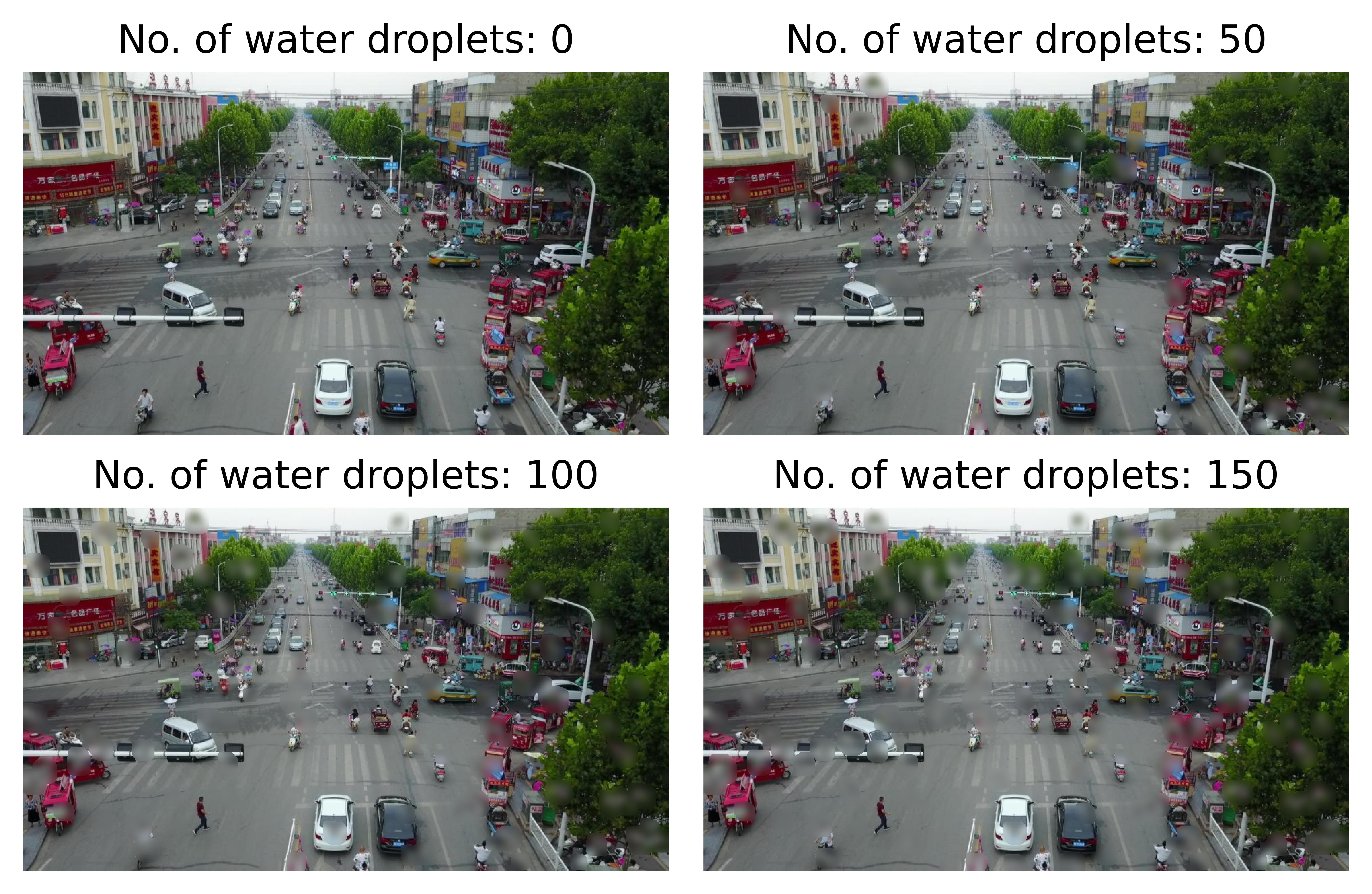
Varying num_drops Parameter

The choice of num_drops values are 0, 50, 100 and 150.

_, ax = plt.subplots(2, 2, figsize=(6, 4), dpi=1200)

for idx in range(0, 4):
    (row, col) = (int(idx / 2), idx % 2)
    num_drops = idx * 50
    perturber = WaterDropletPerturber(num_drops=num_drops, seed=0)
    ax[row, col].set_title(f"No. of water droplets: {num_drops}")
    ax[row, col].imshow(perturber(img_nd_bgr)[0][:, :, ::-1])
    _ = ax[row, col].axis("off")

plt.tight_layout()

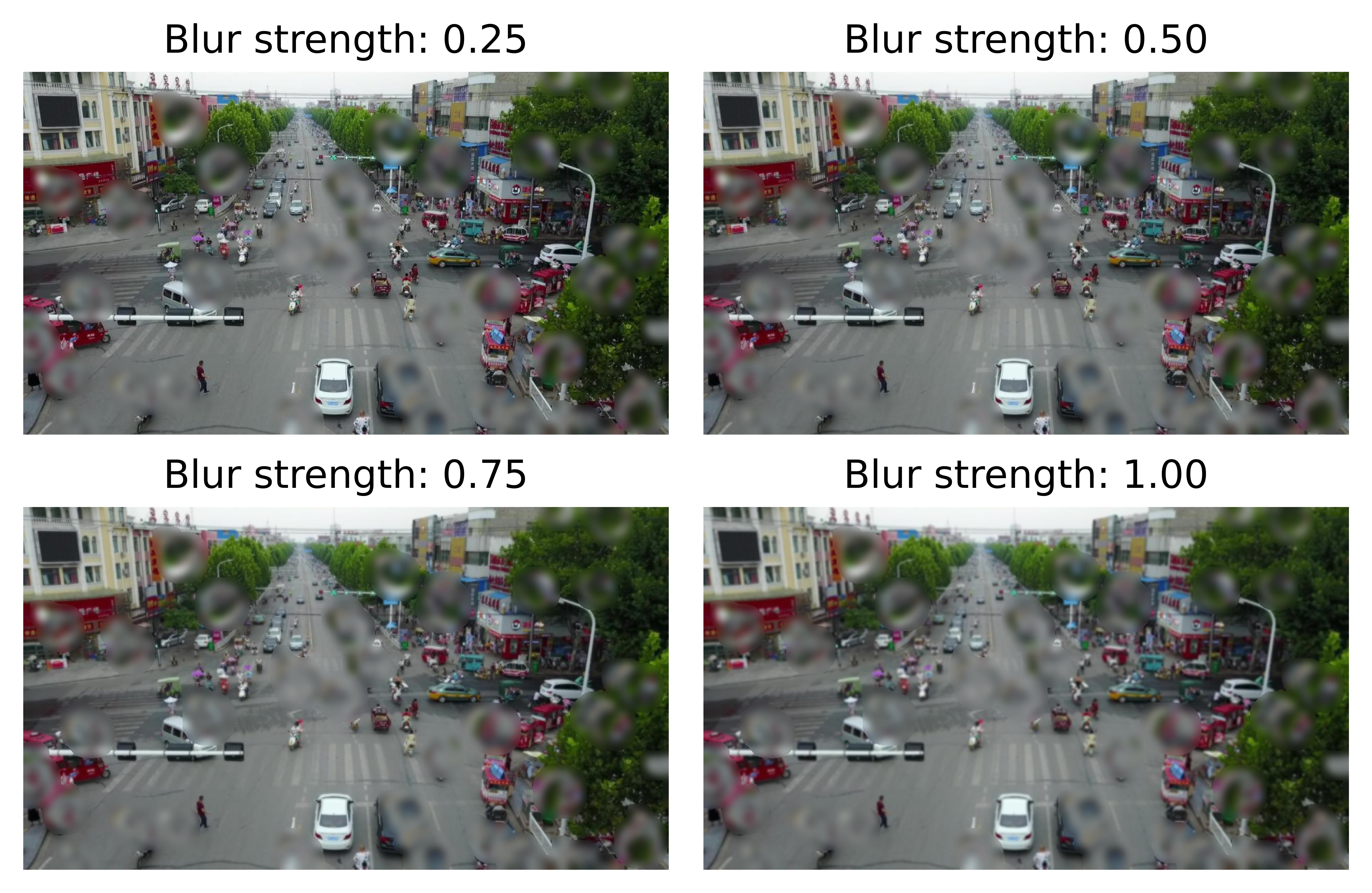
Varying blur_strength Parameter

The choice of blur_strength values are 0.25, 0.5, 0.75 and 1.0.

_, ax = plt.subplots(2, 2, figsize=(6, 4), dpi=1200)

for idx in range(0, 4):
    (row, col) = (int(idx / 2), idx % 2)
    blur_strength = (idx + 1) * 0.25
    perturber = WaterDropletPerturber(size_range=[2.0, 3.0], num_drops=50, blur_strength=blur_strength, seed=0)
    ax[row, col].set_title(f"Blur strength: {blur_strength:.2f}")
    ax[row, col].imshow(perturber(img_nd_bgr)[0][:, :, ::-1])
    _ = ax[row, col].axis("off")

plt.tight_layout()

Baseline Detections

In the next cell, we’ll download a YOLOv11 model, compute object detections on the source image, and display the results. As discussed above, these detections will serve as the “ground truth” for comparisons against the perturbed images.

Note that here, we’re using YOLO’s built-in visualization tool, which automatically adjusts for BGR / RGB order.

# Import YOLO support
import ultralytics

ultralytics.checks()
print("Downloading model...")
model = ultralytics.YOLO("yolo11n.pt")
print("Computing baseline...")
baseline = model(img_nd_bgr)

Ultralytics 8.3.85 🚀 Python-3.9.21 torch-2.7.0+cu126 CUDA:0 (Quadro RTX 5000, 15929MiB)
Setup complete ✅ (40 CPUs, 31.0 GB RAM, 382.4/914.7 GB disk)
Downloading model...
Computing baseline...

0: 384x640 5 persons, 15 cars, 1 motorcycle, 2 trucks, 54.2ms
Speed: 9.3ms preprocess, 54.2ms inference, 284.6ms postprocess per image at shape (1, 3, 384, 640)

MAITE Evaluation Workflow Preparation

We’ll use the MAITE Evaluation workflow to evaluate the performance of the perturbed data against our baseline detections. We’ll need to “wrap” our model, data, and perturbations into callable objects to pass to the maite.tasks.evaluate function:

• We’ll wrap the model to make predictions on input data when called.

• The wrapped dataset will return our test image when called. Note that this will be the original, unperturbed image; we’ll apply our perturbations via…

• …the augmentation object, which applies the perturbation to the image inside the evaluation.

• Finally, the metric object will define our precise scoring methodology.

The evaluation workflow in this notebook is slightly unusual. Typical ML workflows apply many different augmentations / perturbations to much larger datasets, and only call evaluate once to get a statistical view of performance. But since the goal of this notebook is to drill down into how perturbation affects performance, we’ve essentially flipped process, calling evaluate (and thus our wrapped objects) many times, once per loop on our single image perturbed to a known degree, and then observing how the metrics respond.

Some Helper Classes

The following cell adds two classes to allow us to use YOLO detections with the MAITE evaluation workflow:

1. The YOLODetectionTarget helper class that stores the bounding boxes, label indices, and confidence scores for a single image’s detections.

2. The MaiteYOLODetection adapter class that conforms to the MAITE Object Detection Dataset protocol by providing the __len__ and __getitem__ methods. The returned item is a tuple of (image, YOLODetectionTarget, metadata-dictionary).

from dataclasses import dataclass

import torch
from maite.protocols.object_detection import DatumMetadataType

from nrtk.interop.maite.interop.object_detection.dataset import JATICObjectDetectionDataset

##
## Helper class for containing the boxes, label indices, and confidence scores.
##


@dataclass
class YOLODetectionTarget:
    """A helper class to represent object detection results in the format expected by YOLO-based models.

    Attributes:
        boxes (torch.Tensor): A tensor containing the bounding boxes for detected objects in
            [x_min, y_min, x_max, y_max] format.
        labels (torch.Tensor): A tensor containing the class labels for the detected objects.
            These may be floats for compatibility with specific datasets or tools.
        scores (torch.Tensor): A tensor containing the confidence scores for the detected objects.
    """

    boxes: torch.Tensor
    labels: torch.Tensor
    scores: torch.Tensor


##
## Prepare results for ingestion into maite dataset by puttin them into detection object
## Images must be channel first (c, h, w) in maite dataset objects
##
imgs = [np.transpose(img_nd_bgr, (2, 0, 1))]
dets = []
metadata: list[DatumMetadataType] = [{"id": 0}]
for _detection in baseline:
    boxes = baseline[0].boxes.xyxy.cpu()
    labels = baseline[0].boxes.cls.cpu()  # note, these are floats, not ints
    scores = baseline[0].boxes.conf.cpu()

    dets.append(YOLODetectionTarget(boxes, labels, scores))

(1) Wrapping the Detection Model

The first object we’ll wrap will be the detection model. The cell below defines a class adapting YOLO for the MAITE Object Detection Model protocol. The __call__ method runs the model on images in the batch and is called by the MAITE evaluation workflow later in the notebook.

import maite.protocols.object_detection as od
import ultralytics.models
from maite.protocols import ArrayLike, ModelMetadata


class MaiteYOLODetector:
    """A wrapper class for a YOLO model to simplify its usage with input batches and object detection targets.

    This class takes a YOLO model instance, processes input image batches, and converts predictions into
    `YOLODetectionTarget` instances.

    Attributes:
        _model (ultralytics.models.yolo.model.YOLO): The YOLO model instance used for predictions.

    Methods:
        __call__(batch):
            Processes a batch of images through the YOLO model and returns the predictions as
            `YOLODetectionTarget` instances.
    """

    def __init__(self, model: ultralytics.models.yolo.model.YOLO) -> None:
        """Initializes the MaiteYOLODetector with a YOLO model instance.

        Args:
            model (ultralytics.models.yolo.model.YOLO): The YOLO model to use for predictions.
        """
        self._model = model
        # Dummy model metadata type to pass type checking
        self.metadata = ModelMetadata(id="0")

    def __call__(self, batch: Sequence[ArrayLike]) -> Sequence[YOLODetectionTarget]:
        """Processes a batch of images using the YOLO model and converts the predictions to `YOLODetectionTarget`s.

        Args:
            batch (Sequence[ArrayLike]): A batch of images in (c, h, w) format (channel-first).

        Returns:
            Sequence[YOLODetectionTarget]: A list of YOLODetectionTarget instances containing the predictions for each
            image in the batch.
        """
        # Convert images to channel-last format (h, w, c) for YOLO model
        batch_transposed = [np.transpose(batch[i], (1, 2, 0)) for i in range(len(batch))]

        yolo_predictions = self._model(batch_transposed, verbose=False)
        return [
            YOLODetectionTarget(
                p.boxes.xyxy.cpu(),  # Bounding boxes in (x_min, y_min, x_max, y_max) format
                p.boxes.cls.cpu(),  # Class indices for the detected objects
                p.boxes.conf.cpu(),  # Confidence scores for the detections
            )
            for p in yolo_predictions
        ]


# create the wrapped model object
yolo_model: od.Model = MaiteYOLODetector(model)

(2) Wrapping the Dataset

MAITE pairs images and their reference detections (aka targets, ground truth) into datasets. Typical ML workflows have many images per dataset; when these do not all fit in memory simultaneously, a dataloader object is used which can page images and annotations in from disk. For this notebook, however, each invocation of evaluate will use the same single-image dataset (our reference image with its baseline detections.)

# our single image, its baseline detections, and metadata dictionary
# switch image to channel first
single_image_dataset: od.Dataset = JATICObjectDetectionDataset(imgs, dets, metadata, dataset_id="visdrone_ex")

(3) Wrapping the Perturbations as Augmentations

The evaluate function will perturb the image from the dataset using instances of the class defined below, one instance per perturbation value. Note that the object doesn’t perform any augmentations until called by the evaluate workflow.

from nrtk.interop.maite.interop.object_detection.augmentation import JATICDetectionAugmentation

perturber = WaterDropletPerturber(num_drops=0)
identity_augmentation = JATICDetectionAugmentation(perturber, augment_id="identity")

(4) Wrapping the Metrics

We’ll compare the detections in each perturbed image to the unperturbed detections using the Mean Average Precision (mAP) metric from the torchmetrics package. The following cell creates a mAP metrics object, wraps it in a MAITE MAITE Object Detection Metric protocol-compatible class, and then creates an instance of this class, which will be called by evaluate.

This code is copied directly from the MAITE object detection tutorial (with the exception of setting class_metrics=True.)

from maite.protocols import MetricMetadata
from torchmetrics import Metric as TorchMetric
from torchmetrics.detection.mean_ap import MeanAveragePrecision

##
## Create an instance of the MAP metric object
##

tm_metric = MeanAveragePrecision(
    box_format="xyxy",
    iou_type="bbox",
    iou_thresholds=[0.5],
    rec_thresholds=[0.0, 0.1, 0.2, 0.3, 0.4, 0.5, 0.6, 0.7, 0.8, 0.9, 1.0],
    max_detection_thresholds=[1, 10, 100],
    class_metrics=True,
    extended_summary=False,
    average="macro",
)

##
## This wrapper associates the MAP metric object with methods called by the evaluate
## workflow to accumulate detection data and compute the metrics.
##


class WrappedTorchmetricsMetric:
    """A wrapper class for a Torchmetrics metric designed to simplify its usage for object detection tasks.

    This class facilitates the conversion of object detection targets and predictions into the format
    expected by Torchmetrics metrics, allowing for easier integration with existing pipelines.

    Attributes:
        _tm_metric (Callable): The Torchmetrics metric to be wrapped, which takes lists of dictionaries
            containing torch.Tensor objects representing predictions and targets.

    Methods:
        to_tensor_dict(target):
            Converts an `ObjectDetectionTarget` into a dictionary format compatible with the Torchmetrics
            metric's `update` method.

        update(preds, targets):
            Updates the wrapped Torchmetrics metric with batches of predictions and targets in their native format.

        compute():
            Computes the final metric values using the wrapped Torchmetrics metric.

        reset():
            Resets the state of the wrapped Torchmetrics metric.
    """

    def __init__(
        self,
        tm_metric: TorchMetric,
    ) -> None:
        """Initializes the WrappedTorchmetricsMetric with the given Torchmetrics metric.

        Args:
            tm_metric (Callable): A Torchmetrics metric instance that expects predictions and targets as lists of
                dictionaries containing torch.Tensor objects.
        """
        self._tm_metric = tm_metric
        # Dummy metric metadata type to pass type checking
        self.metadata = MetricMetadata(id="0")

    @staticmethod
    def to_tensor_dict(target: od.ObjectDetectionTarget) -> dict[str, torch.Tensor]:
        """Converts an ObjectDetectionTarget into a dictionary format compatible with the Torch's `update` method.

        Args:
            target (od.ObjectDetectionTarget): An object detection target instance containing boxes, labels, and scores.

        Returns:
            dict[str, torch.Tensor]: A dictionary with keys `boxes`, `scores`, and `labels`, each mapping to a tensor.
        """
        return {
            "boxes": torch.as_tensor(target.boxes),
            "scores": torch.as_tensor(target.scores),
            "labels": torch.as_tensor(target.labels).type(torch.int64),
        }

    def update(self, preds: Sequence[od.TargetType], targets: Sequence[od.TargetType]) -> None:
        """Updates the wrapped Torchmetrics metric with the given predictions and targets.

        Args:
            preds (Sequence[od.TargetType]): A batch of predictions in the format expected by the Torchmetrics metric.
            targets (Sequence[od.TargetType]): A batch of targets in the format expected by the Torchmetrics metric.
        """
        preds_tm = [self.to_tensor_dict(pred) for pred in preds]
        targets_tm = [self.to_tensor_dict(tgt) for tgt in targets]
        self._tm_metric.update(preds_tm, targets_tm)

    def compute(self) -> dict[str, Any]:
        """Computes and returns the final metric values using the wrapped Torchmetrics metric.

        Returns:
            dict[str, Any]: A dictionary containing the computed metric values.
        """
        return self._tm_metric.compute()

    def reset(self) -> None:
        """Resets the state of the wrapped Torchmetrics metric, clearing any accumulated data."""
        self._tm_metric.reset()


##
## This is our instance variable that can compute the MAP metrics.
##

mAP_metric: od.Metric = WrappedTorchmetricsMetric(tm_metric)  # noqa: N816

Running the Evaluation

We now have all the wrappings required to evaluate our range of perturbations:

• The yolo_model object, wrapping the YOLO model

• The single_image_dataset object, providing our source image and its baseline detections

• The augmentation object, which when instantiated, applies a single perturbation value to its input

• The mAP_metrics object, defining the metrics to compute at each perturbation value

Evaluation Sanity Check: Ground Truth Against Itself

Here we quickly check the evaluation workflow by creating an identity augmentation (with a num_drops value of 0, leaving the image unchanged) and scoring it. The detections should also be unchanged from the baseline and thus give an mAP of 1.0.

from maite.tasks import evaluate

# call the model for each image in the dataset (in this case, just the source image),
# scoring the resulting detections against those from the dataset
sanity_check_results, _, _ = evaluate(
    model=yolo_model,
    dataset=single_image_dataset,
    augmentation=identity_augmentation,
    metric=mAP_metric,
)

print("Sanity check: overall mAP (should be 1.0):", sanity_check_results["map"].item())

100%|██████████| 1/1 [00:00<00:00, 10.94it/s]

Sanity check: overall mAP (should be 1.0): 0.9772727489471436

Preparing the Data

Now we’ll prepare the augmentation instances for the evaluation. In the cell below, you can set three parameters for sweeping the set of perturbation values:

• sweep_low: the minimum perturbation value (0 has no water droplets)

• sweep_high: the maximum perturbation value (we use something high to see where accuracy will drop to zero)

• sweep_count: how many perturbations to generation

You can also optionally select perturbations to visualize:

• visualization_indices: a list of perturbation indices p, 0 <= p < sweep_count. These instances will be rendered along with their corresponding detections.

SWEEP_LOW = 0
SWEEP_HIGH = 400
SWEEP_COUNT = 21
VISUALIZATION_INDICES = [0, 5, 9]

##
## end user-settable parameters
##

perturbation_values = np.linspace(SWEEP_LOW, SWEEP_HIGH, SWEEP_COUNT, endpoint=True)
augmentations = [
    JATICDetectionAugmentation(
        WaterDropletPerturber(
            size_range=[1.0, 2.0],
            num_drops=int(p),
            seed=0,
        ),
        augment_id=str(idx),
    )
    for idx, p in enumerate(perturbation_values)
]

print(f"Generated {len(augmentations)} perturbation augmentations")

Generated 21 perturbation augmentations

Calling Evaluate on the Augmented Data

We loop over all the augmentations, calling evaluate on each one and building up a list of resulting metrics for analysis.

Any augmentation indices specified above will be rendered in this step.

perturbed_metrics = list()
_, ax = plt.subplots(len(VISUALIZATION_INDICES), figsize=(30, 12), dpi=1200)
for idx, a in enumerate(augmentations):
    # reset the metric object for each dataset
    mAP_metric.reset()
    result, _, _ = evaluate(model=yolo_model, dataset=single_image_dataset, augmentation=a, metric=mAP_metric)
    perturbed_metrics.append(result)

    if idx in VISUALIZATION_INDICES:
        # quickest way is to re-evaluate
        num_drops = a.augment.get_config()["num_drops"]
        print(f"Perturbation #{idx}: No. of droplets={num_drops}")
        datum = single_image_dataset[0]
        batch = ([datum[0]], [datum[1]], [datum[2]])
        # Extract the image from the augmentation and switch it to channel last
        aug = np.transpose(a(batch)[0][0], (1, 2, 0))
        # Plot image
        ax_idx = VISUALIZATION_INDICES.index(idx)
        ax[ax_idx].imshow(model(aug)[0].plot())
        ax[ax_idx].set_title(f"No. of droplets: {num_drops}")
        _ = ax[ax_idx].axis("off")
plt.tight_layout()

  0%|          | 0/1 [00:00<?, ?it/s]

100%|██████████| 1/1 [00:00<00:00, 13.98it/s]

Perturbation #0: No. of droplets=0

100%|██████████| 1/1 [00:17<00:00, 17.08s/it]
100%|██████████| 1/1 [00:31<00:00, 31.72s/it]
100%|██████████| 1/1 [00:47<00:00, 47.09s/it]
100%|██████████| 1/1 [00:58<00:00, 58.92s/it]
100%|██████████| 1/1 [01:05<00:00, 65.80s/it]

Perturbation #5: No. of droplets=100

100%|██████████| 1/1 [01:10<00:00, 70.72s/it]
100%|██████████| 1/1 [01:18<00:00, 78.75s/it]
100%|██████████| 1/1 [01:27<00:00, 87.86s/it]
100%|██████████| 1/1 [01:34<00:00, 94.25s/it]

Perturbation #9: No. of droplets=180

100%|██████████| 1/1 [01:39<00:00, 99.87s/it]
100%|██████████| 1/1 [01:37<00:00, 97.64s/it]
100%|██████████| 1/1 [01:39<00:00, 99.39s/it]
100%|██████████| 1/1 [01:44<00:00, 104.59s/it]
100%|██████████| 1/1 [01:45<00:00, 105.24s/it]
100%|██████████| 1/1 [01:50<00:00, 110.10s/it]
100%|██████████| 1/1 [01:53<00:00, 113.50s/it]
100%|██████████| 1/1 [01:51<00:00, 111.52s/it]
100%|██████████| 1/1 [01:55<00:00, 115.23s/it]
100%|██████████| 1/1 [01:55<00:00, 115.51s/it]
100%|██████████| 1/1 [02:02<00:00, 122.65s/it]

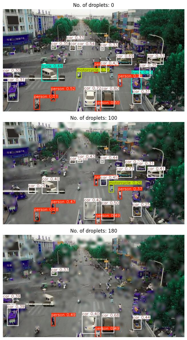
From the above visualizations, we can observe that some of the detections are affected by the surrounding blur even if the object is completely visible. (referring to the No. of droplets: 180 image where the person class example in the center-right is not detected due to the surrounding blur, even though the object is fully visible)

Evaluation Analysis

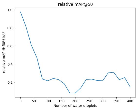
Now we can plot how the metrics (for example, mAP @ IoU=50) vary with perturbation level, keeping in mind this is the mAP scores compared against the detections in the unperturbed image.

map50_list = [m["map_50"].item() for m in perturbed_metrics]
plt.title("mAP@50 on water droplet perturbed dataset")
plt.xlabel("Number of water droplets")
plt.ylabel("mAP @ 50% IoU")
_ = plt.plot(perturbation_values, map50_list)

Evaluation Interpretation

General things to know about mAP calculation:

• The mAP metric calculation does not take into account the images that do not have any detection or any ground truth. In such cases, it returns the default initialization value, -1. It means it couldn’t compute the metric. (Source: link). Hence, in this notebook example, we clip values to a range of [0, 1].

• When having images with no ground truth, the order of those images in the batch can change the mAP calculation. To be more precise, if empty images are at the end of the batch, they will be ignored in the computation. But the empty images that are placed before the last non-empty image are taken into account. (Source: link).

The metric shown, mAP@50, is the average precision of detections across all classes when the bounding box IoU is at least 0.5 (for more details, see here.) The mAP value appears to decrease almost linearly as the number of water droplets increases.

The water droplets’ localized blur effect occludes a lot of objects as the number of droplets increases leading to a drop in the overall mAP value.

Additional Plots

For further insight, we can plot the mAP per class:

#
# Each instance of the metrics object has, potentially, a different set of observed classes.
# Loop through them to accumulate a unified set of classes to ensure consistent plotting across
# all thresholds.
#

unified_classes = set()
for m in perturbed_metrics:
    for class_idx in m["classes"].tolist():
        unified_classes.add(class_idx)

#
# dictionary of class_idx -> list of per-class mAP, or 0 if not present at that threshold
#

class_mAP = {class_idx: list() for class_idx in unified_classes}  # noqa: N816

#
# populate the lists across the perturbation values
#

for m in perturbed_metrics:
    this_perturbation_classes = m["classes"].tolist()
    for class_idx in unified_classes:
        if class_idx in this_perturbation_classes:
            # the index of the class in this individual metric instance
            this_class_idx = this_perturbation_classes.index(class_idx)
            class_map_value = m["map_per_class"][this_class_idx].item()
            # Clip value to 0 if negative
            if class_map_value < 0:
                class_mAP[class_idx].append(0)
            else:
                class_mAP[class_idx].append(m["map_per_class"][this_class_idx].item())
        else:
            class_mAP[class_idx].append(0)

#
# plot
#

plt.title("mAP per class for water droplet perturbed dataset")
plt.xlabel("Number of water droplets")
plt.ylabel("mAP @ 50% IoU")
for class_idx, class_mAP_list in class_mAP.items():  # noqa: N816
    plt.plot(perturbation_values, class_mAP_list, label=baseline[0].names[class_idx])
plt.legend()
plt.show()

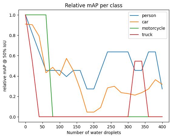
The above plot shows several interesting results regarding water droplet perturbation impacts:

• The person class demonstrates the highest robustness to water droplet perturbations, maintaining better detection performance as droplet count increases.

• The truck and motorcycle classes exhibit the most dramatic decline in mAP scores, showing high sensitivity to water droplet occlusion effects.

• The person and car classes display variable performance that correlates with the spatial distribution and occluded areas created by the water droplets, with detection accuracy fluctuating based on where droplets are positioned relative to these objects.

plt.title("mAP values per area for water droplet perturbed dataset")
plt.xlabel("Number of water droplets")
plt.ylabel("mAP")
for k in ("map", "map_small", "map_medium"):
    plt.plot(perturbation_values, [m[k].item() if m[k].item() >= 0 else 0 for m in perturbed_metrics], label=k)
plt.legend()
plt.show()

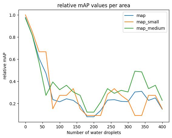
The map line covers all sizes; map_small and map_medium are the mean average precision for objects (smaller than 32^2 pixels, between 32^2 and 96^2 pixels) in area, respectively. (There are no detections in the map_large category.) (Here, the mAP value is averaged over a range of IoU thresholds, between 0.5 and 0.95). The mAP curves across both categories generally follow a similar pattern, but the map_medium category of objects are generally more robust to increasing number of water droplet perturbations.

End of Notebook