Getting Started with NRTK
Overview
NRTK consists of three main parts:
Image Perturbation:
The core of NRTK is based on image perturbation. NRTK offers a wide variety of ways to perturb images and transform bounding boxes. The perturbation classes take an image and perform a transformation based on input parameters. Perturbers implement the PerturbImage interface.
Perturbation Factories:
Building upon image perturbation, perturbation factories are able to take a range of values for parameter(s) and perform multiple perturbations on the same image. This allows for quick and simple generation of multiple perturbations. Perturbation Factories implement the PerturbImageFactory interface.
Model Evaluation:
NRTK provides functionality for evaluating models in the image classification and object detection tasks. The package also provides test orchestration functionality for performing evaluations over a sweep of parameters in order to test model response to varying severity of image degradation. While NRTK perturbations can be used with any evaluation harness, built-in NRTK Generators implement the GenerateObjectDetectorBlackboxResponse interface.
In this example, we’ll generate your first perturbation. Afterwards, the NRTK tutorial provides a deeper look at perturbation and the other main components of NRTK.
Example: A First Look at NRTK Perturbations
Via the pyBSM package, NRTK exposes a large set of Optical Transfer Functions (OTFs). These OTFs can simulate different environmental and sensor-based effects. For example, the JitterOTFPerturber simulates different levels of sensor jitter. By modifying its input parameters, you can observe how sensor jitter affects image quality.
Input Image
Below is an example of an input image that will undergo a Jitter OTF perturbation. This image represents the initial state before any transformation.

Figure 1: Input image.
Code Sample
Below is some example code that applies a Jitter OTF transformation:
from nrtk.impls.perturb_image.pybsm.jitter_otf_perturber import JitterOTFPerturber
import numpy as np
from PIL import Image

INPUT_IMG_FILE = 'docs/images/input.jpg'
image = np.array(Image.open(INPUT_IMG_FILE))

otf = JitterOTFPerturber(s_x=8e-6, s_y=8e-6)
out_image = otf.perturb(image)
This code uses default values and provides a sample input image. However, you can adjust the parameters and use your
own image to visualize the perturbation. The s_x and s_y parameters (the root-mean-squared jitter amplitudes in
radians, in the x and y directions) are the primary way to customize a jitter perturber. Larger jitter amplitudes
generate a larger Gaussian blur kernel. The
how-to guide on OTF perturbations will provide more detail on selecting
specific values for these parameters.
Resulting Image
The output image below shows the effects of the Jitter OTF on the original input. This result illustrates the Gaussian blur introduced due to simulated sensor jitter.
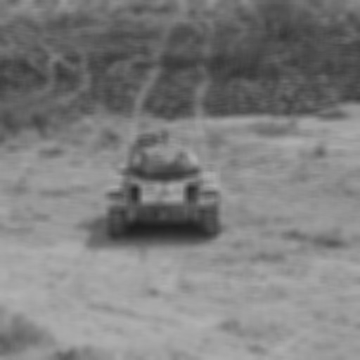
Figure 2: Output image.
Next Steps
For broader context or foundational theory, see:
NRTK Tutorial - Step-by-step tutorial to get started
Concepts of Robustness in Computer Vision - Conceptual guide to NRTK’s architecture and approach
Operational Risk Factors in Computer Vision - Conceptual guide to understand how NRTK’s perturbations map to real-world risk factors