NRTK Tutorial
Introduction
NRTK simplifies jitter data processing for real-time applications, providing tools to analyze and visualize complex datasets. In this tutorial, you’ll learn how to:
Load a sample jitter dataset.
Apply jitter perturbation.
Visualize the results.
By the end of this tutorial, you’ll have a working example that you can expand for your own projects.
Prerequisites
Before starting, ensure the following:
NRTK is installed (see Installation).
Software Requirements: - Python 3.8+ installed. - pip (Python package manager) installed.
Basic Skills: Familiarity with Python programming and using the terminal or command line.
The following sections will guide you through setting up and using an example perturber.
Image Perturbation
The examples
shown below focus on a pyBSM based perturber. To see examples of other perturbations, the
perturbers
notebook shows initialization and use of scikit-image, Pillow, and openCV perturbers.
For this example, we are going to use the PybsmPerturber from pyBSM. This
perturber is useful for creating new images based on existing parameters. The
PybsmSensor and PybsmScenario classes contain the
parameters for an existing sensor and environment, respectively.
import numpy as np
import pybsm
from nrtk.impls.perturb_image.pybsm.scenario import PybsmScenario
from nrtk.impls.perturb_image.pybsm.sensor import PybsmSensor
from nrtk.impls.perturb_image.pybsm.perturber import PybsmPerturber

opt_trans_wavelengths = np.array([0.58-.08,0.58+.08])*1.0e-6
f = 4 #telescope focal length (m)
p = .008e-3  # detector pitch (m)
sensor = PybsmSensor(
    # required
    name                = 'L32511x',
    D                   = 275e-3, # Telescope diameter (m)
    f = f,
    p_x = p,
    opt_trans_wavelengths = opt_trans_wavelengths, #Optical system transmission, red  band first (m)
    # optional
    optics_transmission = 0.5*np.ones(opt_trans_wavelengths.shape[0]), #guess at the full system optical transmission (excluding obscuration)
    eta                 = 0.4, #guess
    w_x                  = p, #detector width is assumed to be equal to the pitch
    w_y                  = p, #detector width is assumed to be equal to the pitch
    int_time            = 30.0e-3, #integration time (s) - this is a maximum, the actual integration time will be, determined by the well fill percentage
    dark_current        = pybsm.dark_current_from_density(1e-5,p,p), #dark current density of 1 nA/cm2 guess, guess mid range for a silicon camera
    read_noise          = 25.0, #rms read noise (rms electrons)
    max_n               = 96000.0, #maximum ADC level (electrons)
    bitdepth            = 11.9, #bit depth
    max_well_fill       = .6, #maximum allowable well fill (see the paper for the logic behind this)
    sx                  = 0.25*p/f, #jitter (radians) - The Olson paper says that its "good" so we'll guess 1/4 ifov rms
    sy                  = 0.25*p/f, #jitter (radians) - The Olson paper says that its "good" so we'll guess 1/4 ifov rms
    dax                 = 100e-6, #drift (radians/s) - again, we'll guess that it's really good
    day                 = 100e-6, #drift (radians/s) - again, we'll guess that it's really good
    qe_wavelengths       = np.array([.3, .4, .5, .6, .7, .8, .9, 1.0, 1.1])*1.0e-6,
    qe                  = np.array([0.05, 0.6, 0.75, 0.85, .85, .75, .5, .2, 0])
)

scenario = PybsmScenario(
        name='niceday',
        ihaze=1, #weather model
        altitude=9000.0, #sensor altitude
        ground_range=0.0, #range to target
        aircraft_speed=100.0
)

perturber=PybsmPerturber(sensor=sensor, scenario=scenario, ground_range=10000)
In the example above, we have created a pyBSM perturber where the output image will have a ground_range of 10000m
instead of 0m. The image below is the original image we will use for future perturbations.
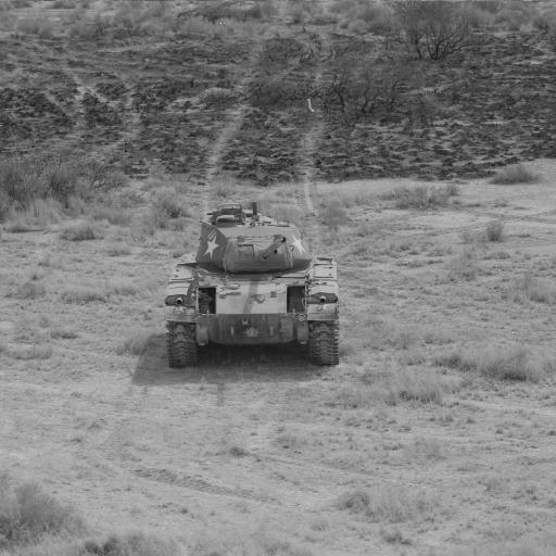
Original image of a tank
The code block below shows the loading of the image above and the calling of the perturber. It is important
to note that the ground sample distance (or img_gsd) is another parameter the user will have to provide.
The resulting image is displayed below the code block.
import cv2

INPUT_IMG_FILE = './data/M-41 Walker Bulldog (USA) width 319cm height 272cm.tiff'
image = cv2.imread(INPUT_IMG_FILE)
img_gsd = 3.19/165.0 #the width of the tank is 319 cm and it spans ~165 pixels in the image

perturbed_image = perturber.perturb(image, additional_params={'img_gsd': img_gsd})
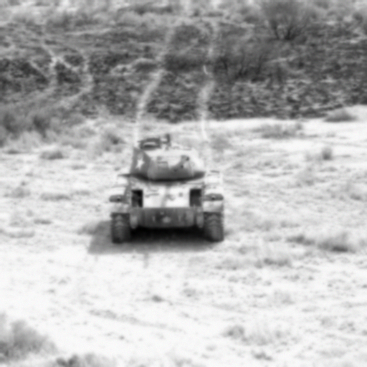
Image of a tank with ground range of 10000m.
Any of the parameters in either PybsmSensor or PybsmScenario can be modified; however, only one parameter can be modified with one value using the basic perturber. The next section will cover modifying multiple parameters and multiple values.
Perturbation Factories
Continuing on from the previous example, the snippet below shows the initialization of a
CustomPybsmPerturbImageFactory. The theta_keys variable controls which parameter(s) we are modifying
and thetas are the actual values of the parameter(s). In this example, we are modifying the
focal length (f) with the values of 1, 2, and 3. The modified images are displayed below the
code block.
from nrtk.impls.perturb_image_factory.pybsm import CustomPybsmPerturbImageFactory

focal_length_pf = CustomPybsmPerturbImageFactory(
    sensor=sensor,
    scenario=scenario,
    theta_keys=["f"],
    thetas=[[1, 2, 3]]
)

for idx, perturber in enumerate(focal_length_pf):
    perturbed_img = perturber(image, additional_params={'img_gsd': img_gsd})
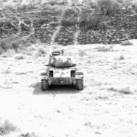
Image of a tank with focal length of 1m. |
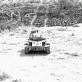
Image of a tank with focal length of 2m. |
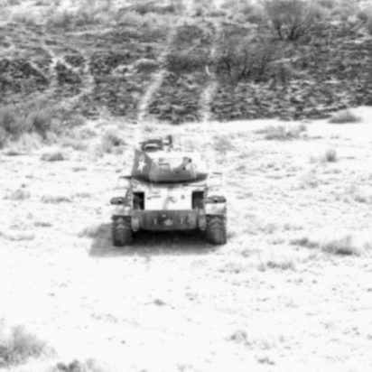
Image of a tank with focal length of 3m.
Not only can you modify multiple values on one parameter, but you can also modify multiple parameters at the same time. The code block below shows the focal length and ground range variables being modified. The resulting images are displayed below the code block.
f_groung_range_pf = CustomPybsmPerturbImageFactory(
    sensor=sensor,
    scenario=scenario,
    theta_keys=["f", "ground_range"],
    thetas=[[1, 2], [10000, 20000]]
)

for idx, perturber in enumerate(f_groung_range_pf):
    perturbed_img = perturber(image, additional_params={'img_gsd': img_gsd})
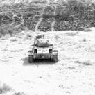
Image of a tank with focal length of 1m and ground range of 10000m. |
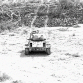
Image of a tank with focal length of 2m and ground range of 10000m. |
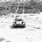
Image of a tank with focal length of 1m and ground range of 20000m. |
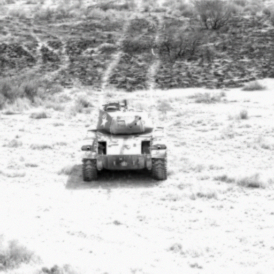
Image of a tank with focal length of 2m and ground range of 20000m. |
Model Evaluation
To see examples of image classification and object detection, the
coco_scorer
notebook from the examples directory shows different scoring techniques. For examples of model response to image
degradations, there are two notebooks to check out. The
simple_generic_generator
notebook shows model response to image degradation through perturbers based on scikit-image, Pillow, and
openCV. The
simple_pybsm_generator
notebook shows model response to image degradation through pyBSM-based perturbers.
Next Steps
Now that you’ve completed this tutorial, you can:
Explore Advanced Features: Try different perturbation methods.
Use Larger Datasets: Test NRTK on real-world jitter logs or larger datasets.
See the How-To section for instructions on Perturbation Visualization Examples.
See the Reference section for code documentation:
See the pyBSM documentation for explanatory information regarding the theory behind perturbations, jitter effects, and the significance of certain parameters matter.